Comparisons and contrasts in emmeans

emmeans package, Version 1.10.5.900003

Contents

This vignette covers techniques for comparing EMMs at levels of a factor predictor, and other related analyses.

1. Pairwise comparisons
2. Other contrasts
3. Formula interface
4. Custom contrasts and linear functions
5. Special behavior with log transformations
6. Interaction contrasts (in “interactions” vignette)
7. Multivariate contrasts (in “interactions” vignette)

Index of all vignette topics

Pairwise comparisons

The most common follow-up analysis for models having factors as predictors is to compare the EMMs with one another. This may be done simply via the pairs() method for emmGrid objects. In the code below, we obtain the EMMs for source for the pigs data, and then compare the sources pairwise.

pigs.lm <- lm(log(conc) ~ source + factor(percent), data = pigs)
pigs.emm.s <- emmeans(pigs.lm, "source")
pairs(pigs.emm.s)

##  contrast    estimate     SE df t.ratio p.value
##  fish - soy    -0.273 0.0529 23  -5.153  0.0001
##  fish - skim   -0.402 0.0542 23  -7.428  <.0001
##  soy - skim    -0.130 0.0530 23  -2.442  0.0570
## 
## Results are averaged over the levels of: percent 
## Results are given on the log (not the response) scale. 
## P value adjustment: tukey method for comparing a family of 3 estimates

In its out-of-the-box configuration, pairs() sets two defaults for summary(): adjust = "tukey" (multiplicity adjustment), and infer = c(FALSE, TRUE) (test statistics, not confidence intervals). You may override these, of course, by calling summary() on the result with different values for these.

In the example above, EMMs for later factor levels are subtracted from those for earlier levels; if you want the comparisons to go in the other direction, use pairs(pigs.emm.s, reverse = TRUE). Also, in multi-factor situations, you may specify by factor(s) to perform the comparisons separately at the levels of those factors.

Matrix displays

The numerical main results associated with pairwise comparisons can be presented compactly in matrix form via the pwpm() function. We simply hand it the emmGrid object to use in making the comparisons:

pwpm(pigs.emm.s)

##        fish    soy   skim
## fish [3.39] <.0001 <.0001
## soy  -0.273 [3.67] 0.0570
## skim -0.402 -0.130 [3.80]
## 
## Row and column labels: source
## Upper triangle: P values   adjust = "tukey"
## Diagonal: [Estimates] (emmean) 
## Lower triangle: Comparisons (estimate)   earlier vs. later

This matrix shows the EMMs along the diagonal, $P$ values in the upper triangle, and the differences in the lower triangle. Options exist to switch off any one of these and to switch which triangle is used for the latter two. Also, optional arguments are passed. For instance, we can reverse the direction of the comparisons, suppress the display of EMMs, swap where the $P$ values go, and perform noninferiority tests with a threshold of 0.05 as follows:

pwpm(pigs.emm.s, means = FALSE, flip = TRUE,     # args for pwpm()
     reverse = TRUE,                             # args for pairs()
     side = ">", delta = 0.05, adjust = "none")  # args for test()

##        fish    soy  skim
## fish         0.273 0.402
## soy  <.0001        0.130
## skim <.0001 0.0013      
## 
## Row and column labels: source
## Lower triangle: P values   side = ">"  delta = 0.05
## Upper triangle: Comparisons (estimate)   later vs. earlier

With all three P values so small, we have fish, soy, and skim in increasing order of noninferiority based on the given threshold.

When more than one factor is present, an existing or newly specified by variables() can split the results into l list of matrices.

Effect size

Some users desire standardized effect-size measures. Most popular is probably Cohen’s d, which is defined as the observed difference, divided by the population SD; and obviously Cohen effect sizes are close cousins of pairwise differences. They are available via the eff_size() function, where the user must specify the emmGrid object with the means to be compared, the estimated population SD sigma, and its degrees of freedom edf. This is illustrated with the current example:

eff_size(pigs.emm.s, sigma = sigma(pigs.lm), edf = 23)

##  contrast    effect.size    SE df lower.CL upper.CL
##  fish - soy        -2.37 0.577 23    -3.56   -1.175
##  fish - skim       -3.49 0.698 23    -4.94   -2.051
##  soy - skim        -1.12 0.490 23    -2.14   -0.112
## 
## Results are averaged over the levels of: percent 
## sigma used for effect sizes: 0.1151 
## Confidence level used: 0.95

The confidence intervals shown take into account the error in estimating sigma as well as the error in the differences. Note that the intervals are narrower if we claim that we know sigma perfectly (i.e., infinite degrees of freedom):

eff_size(pigs.emm.s, sigma = sigma(pigs.lm), edf = Inf)

##  contrast    effect.size    SE df lower.CL upper.CL
##  fish - soy        -2.37 0.460 23    -3.32   -1.418
##  fish - skim       -3.49 0.470 23    -4.47   -2.521
##  soy - skim        -1.12 0.461 23    -2.08   -0.172
## 
## Results are averaged over the levels of: percent 
## sigma used for effect sizes: 0.1151 
## Confidence level used: 0.95

Note that eff_size() expects the object with the means, not the differences. If you want to use the differences, use the method argument to specify that you don’t want to compute pairwise differences again; e.g.,

eff_size(pairs(pigs.emm.s), sigma = sigma(pigs.lm), edf = 23, method = "identity")

(results are identical to the first effect sizes shown).

Graphical comparisons

Comparisons may be summarized graphically via the comparisons argument in plot.emm():

plot(pigs.emm.s, comparisons = TRUE)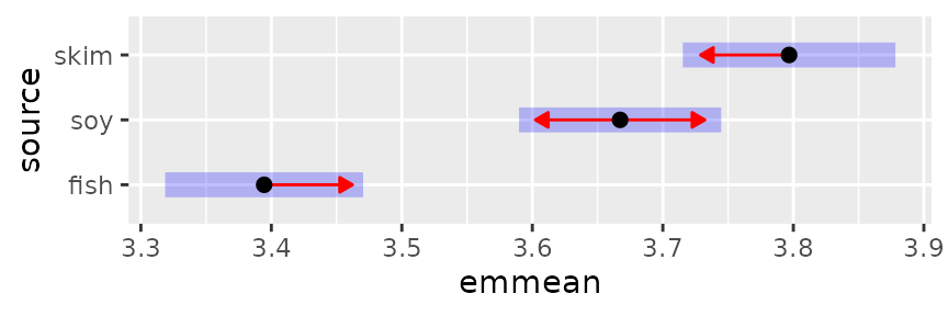

The blue bars are confidence intervals for the EMMs, and the red arrows are for the comparisons among them. If an arrow from one mean overlaps an arrow from another group, the difference is not “significant,” based on the adjust setting (which defaults to "tukey") and the value of alpha (which defaults to 0.05). See the “xplanations” supplement for details on how these are derived.

Note: Don’t ever use confidence intervals for EMMs to perform comparisons; they can be very misleading. Use the comparison arrows instead; or better yet, use pwpp().

A caution: it really is not good practice to draw a bright distinction based on whether or not a P value exceeds some cutoff. This display does dim such distinctions somewhat by allowing the viewer to judge whether a P value is close to alpha one way or the other; but a better strategy is to simply obtain all the P values using pairs(), and look at them individually.

Pairwise P-value plots

In trying to develop an alternative to compact letter displays (see next subsection), we devised the “pairwise P-value plot” displaying all the P values in pairwise comparisons:

pwpp(pigs.emm.s)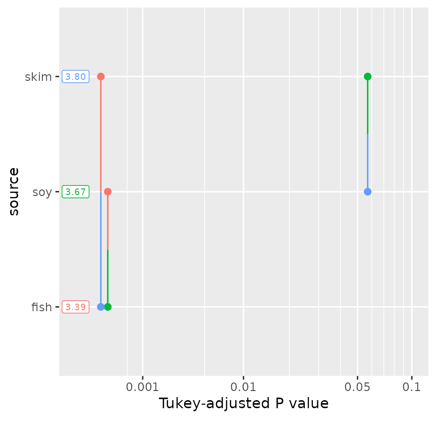

Each comparison is associated with a vertical line segment that joins the scale positions of the two EMMs being compared, and whose horizontal position is determined by the P value of that comparison.

This kind of plot can get quite “busy” as the number of means being compared goes up. For example, suppose we include the interactions in the model for the pigs data, and compare all 12 cell means:

pigs.lmint <- lm(log(conc) ~ source * factor(percent), data = pigs)
pigs.cells <- emmeans(pigs.lmint, ~ source * percent)
pwpp(pigs.cells, type = "response")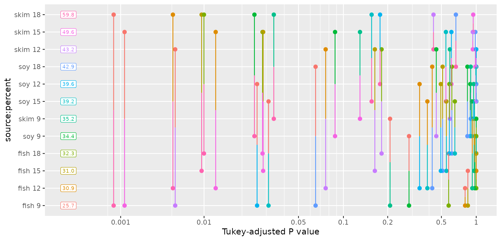

While this plot has a lot of stuff going on, consider looking at it row-by-row. Next to each EMM, we can visualize the P values of all 11 comparisons with each other EMM (along with their color codes). Also, note that we can include arguments that are passed to summary(); in this case, to display the back-transformed means.

If we are willing to forgo the diagonal comparisons (where neither factor has a common level), we can make this a lot less cluttered via a by specification:

pwpp(pigs.cells, by = "source", type = "response")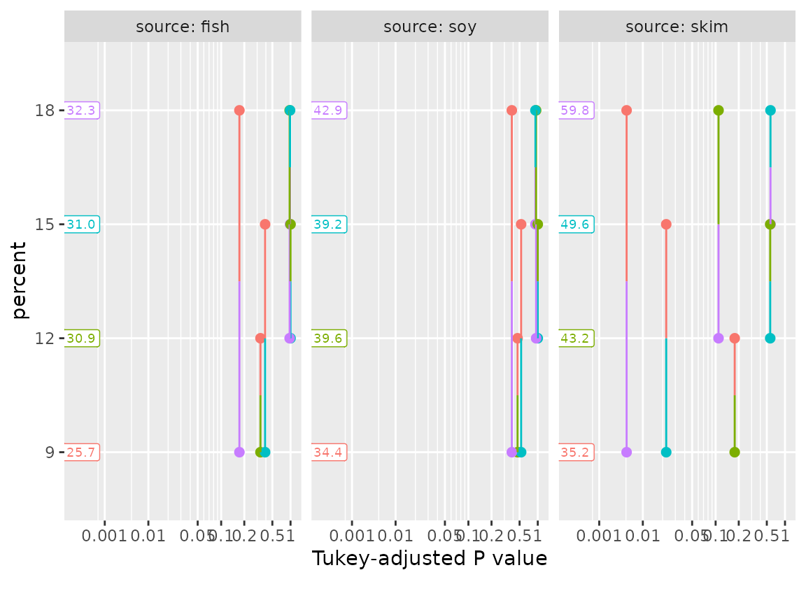

In this latter plot we can see that the comparisons with skim as the source tend to be statistically stronger. This is also an opportunity to remind the user that multiplicity adjustments are made relative to each by group. For example, comparing skim:9 versus skim:15 has a Tukey-adjusted P value somewhat greater than 0.1 when all are in one family of 12 means, but about 0.02 relative to a smaller family of 4 means as depicted in the three-paneled plot.

Compact letter displays (CLDs)

Another way to depict comparisons is by compact letter displays, whereby two EMMs sharing one or more grouping symbols are not “significantly” different. These may be generated by the multcomp::cld() function. I really recommend against this kind of display, though, and decline to illustrate it. These displays promote visually the idea that two means that are “not significantly different” are to be judged as being equal; and that is a very wrong interpretation. In addition, they draw an artificial “bright line” between P values on either side of alpha, even ones that are very close.

Back to Contents

Other contrasts

Pairwise comparisons are an example of linear functions of EMMs. You may use coef() to see the coefficients of these linear functions:

coef(pairs(pigs.emm.s))

##      source c.1 c.2 c.3
## fish   fish   1   1   0
## soy     soy  -1   0   1
## skim   skim   0  -1  -1

The pairwise comparisons correspond to columns of the above results. For example, the first pairwise comparison, fish - soy, gives coefficients of 1, -1, and 0 to fish, soy, and skim, respectively. In cases, such as this one, where each column of coefficients sums to zero, the linear functions are termed contrasts

The contrast() function provides for general contrasts (and linear functions, as well) of factor levels. Its second argument, method, is used to specify what method is to be used. In this section we describe the built-in ones, where we simply provide the name of the built-in method. Consider, for example, the factor percent in the model pigs.lm . It is treated as a factor in the model, but it corresponds to equally-spaced values of a numeric variable. In such cases, users often want to compute orthogonal polynomial contrasts:

pigs.emm.p <- emmeans(pigs.lm, "percent")
ply <- contrast(pigs.emm.p, "poly")
ply

##  contrast  estimate     SE df t.ratio p.value
##  linear      0.9374 0.2110 23   4.452  0.0002
##  quadratic  -0.0971 0.0883 23  -1.099  0.2830
##  cubic       0.1863 0.1880 23   0.992  0.3313
## 
## Results are averaged over the levels of: source 
## Results are given on the log (not the response) scale.

coef(ply)

##           percent c.1 c.2 c.3
## percent9        9  -3   1  -1
## percent12      12  -1  -1   3
## percent15      15   1  -1  -3
## percent18      18   3   1   1

We obtain tests for the linear, quadratic, and cubic trends. The coefficients are those that can be found in tables in many experimental-design texts. It is important to understand that the estimated linear contrast is not the slope of a line fitted to the data. It is simply a contrast having coefficients that increase linearly. It does test the linear trend, however.

There are a number of other named contrast methods, for example "trt.vs.ctrl", "eff", and "consec". The "pairwise" and "revpairwise" methods in contrast() are the same as Pairs() and pairs(..., reverse = TRUE). See help("contrast-methods") for details.

Back to Contents

Formula interface

If you already know what contrasts you will want before calling emmeans(), a quick way to get them is to specify the method as the left-hand side of the formula in its second argument. For example, with the oranges dataset provided in the package,

org.aov <- aov(sales1 ~ day + Error(store), data = oranges,
               contrasts = list(day = "contr.sum"))
org.emml <- emmeans(org.aov, consec ~ day)
org.emml

## $emmeans
##  day emmean   SE   df lower.CL upper.CL
##  1     7.87 2.77 29.2     2.21     13.5
##  2     7.10 2.77 29.2     1.43     12.8
##  3    13.76 2.77 29.2     8.09     19.4
##  4     8.04 2.77 29.2     2.37     13.7
##  5    12.92 2.77 29.2     7.26     18.6
##  6    11.60 2.77 29.2     5.94     17.3
## 
## Warning: EMMs are biased unless design is perfectly balanced 
## Confidence level used: 0.95 
## 
## $contrasts
##  contrast    estimate   SE df t.ratio p.value
##  day2 - day1   -0.772 3.78 25  -0.204  0.9997
##  day3 - day2    6.658 3.78 25   1.763  0.3241
##  day4 - day3   -5.716 3.78 25  -1.513  0.4679
##  day5 - day4    4.882 3.78 25   1.293  0.6128
##  day6 - day5   -1.321 3.78 25  -0.350  0.9965
## 
## P value adjustment: mvt method for 5 tests

The contrasts shown are the day-to-day changes.

This two-sided formula technique is quite convenient, but it can also create confusion. For one thing, the result is not an emmGrid object anymore; it is a list of emmGrid objects, called an emm_list. You may need to be cognizant of that if you are to do further contrasts or other analyzes. For example if you want "eff" contrasts as well, you need to do contrast(org.emml[[1]], "eff") or contrast(org.emml, "eff", which = 1).

Another issue is that it may be unclear which part of the results is affected by certain options. For example, if you were to add adjust = "bonf" to the org.emm call above, would the Bonferroni adjustment be applied to the EMMs, or to the contrasts? (See the documentation if interested; but the best practice is to avoid such dilemmas.)

Back to Contents

Custom contrasts and linear functions

The user may write a custom contrast function for use in contrast(). What’s needed is a function having the desired name with ".emmc" appended, that generates the needed coefficients as a list or data frame. The function should take a vector of levels as its first argument, and any optional parameters as additional arguments. It should also always have a ... argument to allow for unspecified arguments that may occur in the call.

As an example, suppose we want to compare every third level of a treatment. The following function provides for this:

skip_comp.emmc <- function(levels, skip = 1, reverse = FALSE, ...) {
    if((k <- length(levels)) < skip + 1)
        stop("Need at least ", skip + 1, " levels")
    coef <- data.frame()
    coef <- as.data.frame(lapply(seq_len(k - skip - 1), function(i) {
        sgn <- ifelse(reverse, -1, 1)
        sgn * c(rep(0, i - 1), 1, rep(0, skip), -1, rep(0, k - i - skip - 1))
    }))
    names(coef) <- sapply(coef, function(x)
        paste(which(x == 1), "-", which(x == -1)))
    attr(coef, "adjust") = "fdr"   # default adjustment method
    coef
}

To test it, try 5 levels:

skip_comp.emmc(1:5)

##   1 - 3 2 - 4 3 - 5
## 1     1     0     0
## 2     0     1     0
## 3    -1     0     1
## 4     0    -1     0
## 5     0     0    -1

skip_comp.emmc(1:5, skip = 0, reverse = TRUE)

##   2 - 1 3 - 2 4 - 3 5 - 4
## 1    -1     0     0     0
## 2     1    -1     0     0
## 3     0     1    -1     0
## 4     0     0     1    -1
## 5     0     0     0     1

(The latter is the same as "consec" contrasts.) Now try it with the oranges example we had previously:

contrast(org.emml[[1]], "skip_comp", skip = 2, reverse = TRUE)

##  contrast estimate   SE df t.ratio p.value
##  4 - 1        0.17 3.78 25   0.045  0.9645
##  5 - 2        5.82 3.78 25   1.542  0.4069
##  6 - 3       -2.15 3.78 25  -0.571  0.8601
## 
## P value adjustment: fdr method for 3 tests

The contrast() function may in fact be used to compute arbitrary linear functions of EMMs. Suppose for some reason we want to estimate the quantities $\lambda_1 = \mu_1+2\mu_2-7$ and $\lambda_2 = 3\mu_2-2\mu_3+1$, where the $\mu_j$ are the population values of the source EMMs in the pigs example. This may be done by providing the coefficients in a list, and the added constants in the offset argument:

LF <- contrast(pigs.emm.s, 
               list(lambda1 = c(1, 2, 0), lambda2 = c(0, 3, -2)),
               offset = c(-7, 1))
confint(LF, adjust = "bonferroni")

##  contrast estimate     SE df lower.CL upper.CL
##  lambda1      3.73 0.0827 23     3.53     3.93
##  lambda2      4.41 0.1340 23     4.09     4.73
## 
## Results are averaged over the levels of: percent 
## Note: contrasts are still on the log scale. Consider using
##       regrid() if you want contrasts of back-transformed estimates. 
## Confidence level used: 0.95 
## Conf-level adjustment: bonferroni method for 2 estimates

Back to Contents

Special properties of log (and logit) transformations

Suppose we obtain EMMs for a model having a response transformation or link function. In most cases, when we compute contrasts of those EMMs, there is no natural way to express those contrasts on anything other than the transformed scale. For example, in a model fitted using glm() with the gamma() family, the default link function is the inverse. Predictions on such a model are estimates of $1/\mu_j$ for various $j$. Comparisons of predictions will be estimates of $1/\mu_j - 1/\mu_{k}$ for $j \ne k$. There is no natural way to back-transform these differences to some other interpretable scale.

However, logs are an exception, in that $\log\mu_j - \log\mu_k = \log(\mu_j/\mu_k)$. Accordingly, when contrast() (or pairs()) notices that the response is on the log scale, it back-transforms contrasts to ratios when results are to be of response type. For example:

pairs(pigs.emm.s, type = "lp")

##  contrast    estimate     SE df t.ratio p.value
##  fish - soy    -0.273 0.0529 23  -5.153  0.0001
##  fish - skim   -0.402 0.0542 23  -7.428  <.0001
##  soy - skim    -0.130 0.0530 23  -2.442  0.0570
## 
## Results are averaged over the levels of: percent 
## Results are given on the log (not the response) scale. 
## P value adjustment: tukey method for comparing a family of 3 estimates

pairs(pigs.emm.s, type = "response")

##  contrast    ratio     SE df null t.ratio p.value
##  fish / soy  0.761 0.0403 23    1  -5.153  0.0001
##  fish / skim 0.669 0.0362 23    1  -7.428  <.0001
##  soy / skim  0.879 0.0466 23    1  -2.442  0.0570
## 
## Results are averaged over the levels of: percent 
## P value adjustment: tukey method for comparing a family of 3 estimates 
## Tests are performed on the log scale

As is true of EMM summaries with type = "response", the tests and confidence intervals are done before back-transforming. The ratios estimated here are actually ratios of geometric means. In general, a model with a log response is in fact a model for relative effects of any of its linear predictors, and this back-transformation to ratios goes hand-in-hand with that.

In generalized linear models, this behaviors will occur in two common cases: Poisson or count regression, for which the usual link is the log; and logistic regression, because logits are logs of odds ratios.

Back to Contents

Index of all vignette topics