Prediction in **emmeans**

emmeans package, Version 1.10.5.900003

In this vignette, we discuss emmeans’s rudimentary capabilities for constructing prediction intervals.

Contents

1. Focus on reference grids
2. Need for an SD estimate
3. Feedlot example
4. Predictions on particular strata
5. Predictions with Bayesian models

Index of all vignette topics

Focus on reference grids

Prediction is not the central purpose of the emmeans package. Even its name refers to the idea of obtaining marginal averages of fitted values; and it is a rare situation where one would want to make a prediction of the average of several observations. We can certainly do that if it is truly desired, but almost always, predictions should be based on the reference grid itself (i.e., not the result of an emmeans() call), inasmuch as a reference grid comprises combinations of model predictors.

Need for an SD estimate

A prediction interval requires an estimate of the error standard deviation, because we need to account for both the uncertainty of our point predictions and the uncertainty of outcomes centered on those estimates. By its current design, we save the value (if any) returned by stats::sigma(object) when a reference grid is constructed for a model object. Not all models provide a sigma() method, in which case an error is thrown if the error SD is not manually specified. Also, in many cases, there may be a sigma() method, but it does not return the appropriate value(s) in the context of the needed predictions. (In an object returned by lme4::glmer(), for example,sigma()` seems to always returns 1.0.) Indeed, as will be seen in the example that follows, one usually needs to construct a manual SD estimate when the model is a mixed-effects model.

So it is essentially always important to think very specifically about whether we are using an appropriate value. You may check the value being assumed by looking at the misc slot in the reference grid:

rg <- ref_grid(model)
rg@misc$sigma

Finally, sigma may be a vector, as long as it is conformable with the estimates in the reference grid. This would be appropriate, for example, with a model fitted by nlme::gls() with some kind of non-homogeneous error structure. It may take some effort, as well as a clear understanding of the model and its structure, to obtain suitable SD estimates. It was suggested to me that the function insight::get_variance() may be helpful – especially when working with an unfamiliar model class. Personally, I prefer to make sure I understand the structure of the model object and/or its summary to ensure I am not going astray.

Back to Contents

Feedlot example

To illustrate, consider the feedlot dataset provided with the package. Here we have several herds of feeder cattle that are sent to feed lots and given one of three diets. The weights of the cattle are measured at time of entry (ewt) and at time of slaughter (swt). Different herds have possibly different entry weights, based on breed and ranching practices, so we will center each herd’s ewt measurements, then use that as a covariate in a mixed model:

feedlot = transform(feedlot, adj.ewt = ewt - predict(lm(ewt ~ herd)))
require(lme4)
feedlot.lmer <- lmer(swt ~ adj.ewt + diet + (1|herd), data = feedlot)
feedlot.rg <- ref_grid(feedlot.lmer, at = list(adj.ewt = 0))
summary(feedlot.rg)  ## point predictions

##  adj.ewt diet   prediction   SE   df
##        0 Low          1029 25.5 12.0
##        0 Medium        998 26.4 13.7
##        0 High         1031 29.4 19.9
## 
## Degrees-of-freedom method: kenward-roger

Now, as advised, let’s look at the SDs involved in this model:

lme4::VarCorr(feedlot.lmer)  ## for the model

##  Groups   Name        Std.Dev.
##  herd     (Intercept) 77.087  
##  Residual             57.832

feedlot.rg@misc$sigma  ## default in the ref. grid

## [1] 57.83221

So the residual SD will be assumed in our prediction intervals if we don’t specify something else. And we do want something else, because in order to predict the slaughter weight of an arbitrary animal, without regard to its herd, we need to account for the variation among herds too, which is seen to be considerable. The two SDs reported by VarCorr() are assumed to represent independent sources of variation, so they may be combined into a total SD using the Pythagorean Theorem. We will update the reference grid with the new value:

feedlot.rg <- update(feedlot.rg, sigma = sqrt(77.087^2 + 57.832^2))

We are now ready to form prediction intervals. To do so, simply call the predict() function with an interval argument:

predict(feedlot.rg, interval = "prediction")

##  adj.ewt diet   prediction    SE   df lower.PL upper.PL
##        0 Low          1029  99.7 12.0      812     1247
##        0 Medium        998  99.9 13.7      783     1213
##        0 High         1031 101.0 19.9      821     1241
## 
## Degrees-of-freedom method: kenward-roger 
## Prediction intervals and SEs are based on an error SD of 96.369 
## Confidence level used: 0.95

These results may also be displayed graphically:

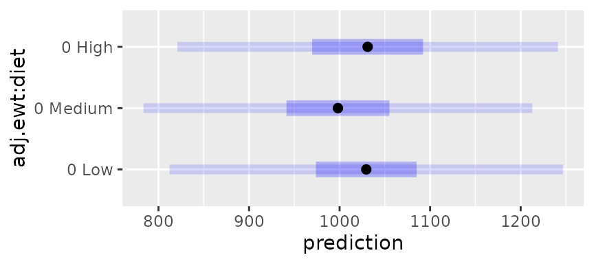
plot(feedlot.rg, PIs = TRUE)

The inner intervals are confidence intervals, and the outer ones are the prediction intervals.

Note that the SEs for prediction are considerably greater than the SEs for estimation in the original summary of feedlot.rg. Also, as a sanity check, observe that these prediction intervals cover about the same ground as the original data:

range(feedlot$swt)

## [1]  816 1248

By the way, we could have specified the desired sigma value as an additional sigma argument in the predict() call, rather than updating the feedlot.rg object.

Back to Contents

Predictions on particular strata

Suppose, in our example, we want to predict swt for one or more particular herds. Then the total SD we computed is not appropriate for that purpose, because that includes variation among herds.

But more to the point, if we are talking about particular herds, then we are really regarding herd as a fixed effect of interest; so the expedient thing to do is to fit a different model where herd is a fixed effect:

feedlot.lm <- lm(swt ~ adj.ewt + diet + herd, data = feedlot)

So to predict slaughter weight for herds 9 and 19:

newrg <- ref_grid(feedlot.lm, at = list(adj.ewt = 0, herd = c("9", "19")))
predict(newrg, interval = "prediction", by = "herd")

## herd = 9:
##  adj.ewt diet   prediction   SE df lower.PL upper.PL
##        0 Low           867 63.6 53      740      995
##        0 Medium        835 64.1 53      707      964
##        0 High          866 66.3 53      733      999
## 
## herd = 19:
##  adj.ewt diet   prediction   SE df lower.PL upper.PL
##        0 Low          1069 62.1 53      945     1194
##        0 Medium       1037 62.8 53      911     1163
##        0 High         1068 64.0 53      940     1197
## 
## Prediction intervals and SEs are based on an error SD of 57.782 
## Confidence level used: 0.95

This is an instance where the default sigma was already correct (being the only error SD we have available). The SD value is comparable to the residual SD in the previous model, and the prediction SEs are smaller than those for predicting over all herds.

Back to Contents

Predictions with Bayesian models

For models fitted using Bayesian methods, these kinds of prediction intervals are available only by forcing a frequentist analysis (frequentist = TRUE).

However, a better and more flexible approach with Bayesian models is to simulate observations from the posterior predictive distribution. This is done via as.mcmc() and specifying a likelihood argument. An example is given in the “sophisticated models” vignette.

Back to Contents

Index of all vignette topics