Transformations and link functions in emmeans

emmeans package, Version 1.10.6.90002

Contents

This vignette covers the intricacies of transformations and link functions in emmeans.

1. Overview
2. Re-gridding
3. Link functions
4. Graphing transformations and links
5. Both a response transformation and a link
6. Special transformations
7. Specifying a transformation after the fact
8. Auto-detected transformations
9. Standardized response
10. Faking a log transformation
    1. Faking other transformations
    2. Alternative scale
11. Bias adjustment

Index of all vignette topics

Overview

Consider an example with the pigs dataset that is used in many of these vignettes; but this time, we use a log transformation of the response:

pigs.lm <- lm(log(conc) ~ source + factor(percent), data = pigs)

This model has two factors, source and percent (coerced to a factor), as predictors; and log-transformed conc as the response. Here we obtain the EMMs for source, examine its structure, and finally produce a summary, including a test against a null value of log(35):

emm.src <- emmeans(pigs.lm, "source")
str(emm.src)

## 'emmGrid' object with variables:
##     source = fish, soy, skim
## Transformation: "log"

summary(emm.src, infer = TRUE, null = log(35))

##  source emmean     SE df lower.CL upper.CL null t.ratio p.value
##  fish     3.39 0.0367 23     3.32     3.47 3.56  -4.385  0.0002
##  soy      3.67 0.0374 23     3.59     3.74 3.56   2.988  0.0066
##  skim     3.80 0.0394 23     3.72     3.88 3.56   6.130  <.0001
## 
## Results are averaged over the levels of: percent 
## Results are given on the log (not the response) scale. 
## Confidence level used: 0.95

Now suppose that we want the EMMs expressed on the same scale as conc. This can be done by adding type = "response" to the summary() call:

summary(emm.src, infer = TRUE, null = log(35), type = "response")

##  source response   SE df lower.CL upper.CL null t.ratio p.value
##  fish       29.8 1.09 23     27.6     32.1   35  -4.385  0.0002
##  soy        39.1 1.47 23     36.2     42.3   35   2.988  0.0066
##  skim       44.6 1.75 23     41.1     48.3   35   6.130  <.0001
## 
## Results are averaged over the levels of: percent 
## Confidence level used: 0.95 
## Intervals are back-transformed from the log scale 
## Tests are performed on the log scale

Note: Looking ahead, this output is compared later in this vignette with a bias-adjusted version.

Timing is everything

Dealing with transformations in emmeans is somewhat complex, due to the large number of possibilities. But the key is understanding what happens, when. These results come from a sequence of steps. Here is what happens (and doesn’t happen) at each step:

1. The reference grid is constructed for the log(conc) model. The fact that a log transformation is used is recorded, but nothing else is done with that information.
2. The predictions on the reference grid are averaged over the four percent levels, for each source, to obtain the EMMs for source – still on the log(conc) scale.
3. The standard errors and confidence intervals for these EMMs are computed – still on the log(conc) scale.
4. Only now do we do back-transformation…
   1. The EMMs are back-transformed to the conc scale.
   2. The endpoints of the confidence intervals are back-transformed.
   3. The t tests and P values are left as-is.
   4. The standard errors are converted to the conc scale using the delta method. These SEs were not used in constructing the tests and confidence intervals.

The model is our best guide

This choice of timing is based on the idea that the model is right. In particular, the fact that the response is transformed suggests that the transformed scale is the best scale to be working with. In addition, the model specifies that the effects of source and percent are linear on the transformed scale; inasmuch as marginal averaging to obtain EMMs is a linear operation, that averaging is best done on the transformed scale. For those two good reasons, back-transforming to the response scale is delayed until the very end by default.

Back to Contents

Re-gridding

As well-advised as it is, some users may not want the default timing of things. The tool for changing when back-transformation is performed is the regrid() function – which, with default settings of its arguments, back-transforms an emmGrid object and adjusts everything in it appropriately. For example:

str(regrid(emm.src))

## 'emmGrid' object with variables:
##     source = fish, soy, skim

summary(regrid(emm.src), infer = TRUE, null = 35)

##  source response   SE df lower.CL upper.CL null t.ratio p.value
##  fish       29.8 1.09 23     27.5     32.1   35  -4.758  0.0001
##  soy        39.1 1.47 23     36.1     42.2   35   2.827  0.0096
##  skim       44.6 1.75 23     40.9     48.2   35   5.446  <.0001
## 
## Results are averaged over the levels of: percent 
## Confidence level used: 0.95

Notice that the structure no longer includes the transformation. That’s because it is no longer relevant; the reference grid is on the conc scale, and how we got there is now forgotten. Compare this summary() result with the preceding one, and note the following:

• It no longer has annotations concerning transformations.
• The estimates and SEs are identical.
• The confidence intervals, t ratios, and P values are not identical. This is because, this time, the SEs shown in the table are the ones actually used to construct the tests and intervals.

Understood, right? But think carefully about how these EMMs were obtained. They are back-transformed from emm.src, in which the marginal averaging was done on the log scale. If we want to back-transform before doing the averaging, we need to call regrid() after the reference grid is constructed but before the averaging takes place:

pigs.rg <- ref_grid(pigs.lm)
remm.src <- emmeans(regrid(pigs.rg), "source")
summary(remm.src, infer = TRUE, null = 35)

##  source response   SE df lower.CL upper.CL null t.ratio p.value
##  fish       30.0 1.10 23     27.7     32.2   35  -4.585  0.0001
##  soy        39.4 1.49 23     36.3     42.5   35   2.927  0.0076
##  skim       44.8 1.79 23     41.1     48.5   35   5.486  <.0001
## 
## Results are averaged over the levels of: percent 
## Confidence level used: 0.95

These results all differ from either of the previous two summaries – again, because the averaging is done on the conc scale rather than the log(conc) scale.

Note: For those who want to routinely back-transform before averaging, the regrid argument in ref_grid() simplifies this. The first two steps above could have been done more easily as follows:

remm.src <- emmeans(pigs.lm, "source", regrid = "response")

But don’t get regrid and type confused. The regrid argument is passed to regrid() (as the transform argument) after the reference grid is constructed, whereas the type argument is simply remembered and used by summary(). So a similar-looking call:

emmeans(pigs.lm, "source", type = "response")

will compute the results we have seen for emm.src – back-transformed after averaging on the log scale.

Remember again: When it comes to transformations, timing is everything.

Implied regridding with certain modes

Some model classes provide special argument(s) (typically mode) that may cause transformations or links to be handled early. For example, cumulative link models for ordinal data allow for a "prob" mode that produces estimates of probabilities for each ordinal level. The reference grid comprises estimates on a probability scale, and whatever link was used (say, probit) has already been accounted for, so is not “remembered” for possible later back-transformation. In that sense, when we use mode = "prob", it is sort of like an implied call to regrid() that takes place at the time the reference grid is constructed, preempting any timing choices you might otherwise have made about handling the transformation. If there are one or more factors that are averaged over in estimating marginal means will be averages of the probabilities in the reference grid; so they will be different than what you would have obtained by keeping things on the link scale and then computing the probabilities after averaging on the link scale.

Similar things happen with certain options with multinomial models, zero-inflated, or hurdle models. Those special modes are a great convenience for getting estimates on a scale that is desired, but they also force you to obtain marginal means of measurements already on that scale.

Back to Contents

Link functions

Exactly the same ideas we have presented for response transformations apply to generalized linear models having non-identity link functions. As far as emmeans is concerned, there is no difference at all.

To illustrate, consider the neuralgia dataset provided in the package. These data come from an experiment reported in a SAS technical report where different treatments for neuralgia are compared. The patient’s sex is an additional factor, and their age is a covariate. The response is Pain, a binary variable on whether or not the patient reports neuralgia pain after treatment. The model suggested in the SAS report is equivalent to the following. We use it to obtain estimated probabilities of experiencing pain:

neuralgia.glm <- glm(Pain ~ Treatment * Sex + Age, family = binomial(), data = neuralgia)
neuralgia.emm <- emmeans(neuralgia.glm, "Treatment", type = "response")

## NOTE: Results may be misleading due to involvement in interactions

neuralgia.emm

##  Treatment  prob     SE  df asymp.LCL asymp.UCL
##  A         0.211 0.1110 Inf    0.0675     0.497
##  B         0.121 0.0835 Inf    0.0285     0.391
##  P         0.866 0.0883 Inf    0.5927     0.966
## 
## Results are averaged over the levels of: Sex 
## Confidence level used: 0.95 
## Intervals are back-transformed from the logit scale

(The note about the interaction is discussed shortly.) Note that the averaging over Sex is done on the logit scale, before the results are back-transformed for the summary. We may use pairs() to compare these estimates; note that logits are logs of odds; so this is another instance where log-differences are back-transformed – in this case to odds ratios:

pairs(neuralgia.emm, reverse = TRUE)

##  contrast odds.ratio     SE  df null z.ratio p.value
##  B / A         0.513  0.515 Inf    1  -0.665  0.7837
##  P / A        24.234 25.100 Inf    1   3.073  0.0060
##  P / B        47.213 57.200 Inf    1   3.179  0.0042
## 
## Results are averaged over the levels of: Sex 
## P value adjustment: tukey method for comparing a family of 3 estimates 
## Tests are performed on the log odds ratio scale

So there is evidence of considerably more pain being reported with placebo (treatment P) than with either of the other two treatments. The estimated odds of pain with B are about half that for A, but this finding is not statistically significant. (The odds that this is a made-up dataset seem quite high, but that finding is strictly this author’s impression.)

Observe that there is a note in the output for neuralgia.emm that the results may be misleading. It is important to take it seriously, because if two factors interact, it may be the case that marginal averages of predictions don’t reflect what is happening at any level of the factors being averaged over. To find out, look at an interaction plot of the fitted model:

emmip(neuralgia.glm, Sex ~ Treatment)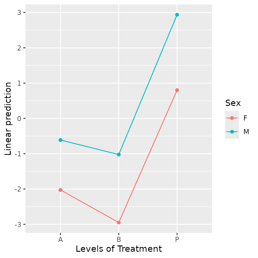

## Error in get(paste0(generic, ".", class), envir = get_method_env()) : 
##   object 'type_sum.accel' not found

There is no practical difference between females and males in the patterns of response to Treatment; so I think most people would be quite comfortable with the marginal results that are reported here.

Some users prefer risk ratios (ratios of probabilities) rather than odds ratios. We will revisit this example below after we have discussed some more tools.

Back to Contents

Graphing transformations and links

There are a few options for displaying transformed results graphically. First, the type argument works just as it does in displaying a tabular summary. Following through with the neuralgia example, let us display the marginal Treatment EMMs on both the link scale and the response scale (we are opting to do the averaging on the link scale):

neur.Trt.emm <- suppressMessages(emmeans(neuralgia.glm, "Treatment"))
plot(neur.Trt.emm)   # Link scale by default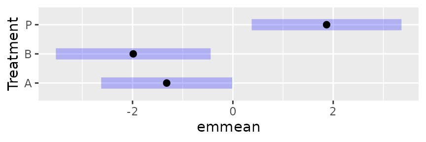

plot(neur.Trt.emm, type = "response")

<img src=“/home/runner/work/emmeans/emmeans/docs/articles/transformations_files/figure-html/unnamed-chunk-13-2.png” alt=“Plot B: Display of the results of confint(neur.Trt.emm, type =”response”). These intervals are markedly skewed right|left for low|high estimated probabilities” width=“432” />

Besides whether or not we see response values, there is a dramatic difference in the symmetry of the intervals.

For emmip() and plot() only (and currently only with the “ggplot” engine), there is also the option of specifying type = "scale", which causes the response values to be calculated but plotted on a nonlinear scale corresponding to the transformation or link:

plot(neur.Trt.emm, type = "scale")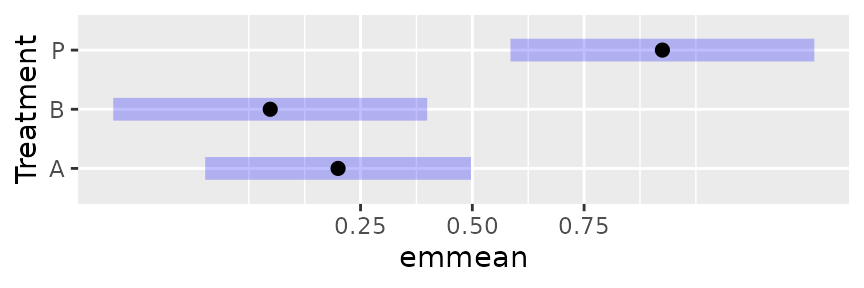

Notice that the interior part of this plot is identical to the plot on the link scale. Only the horizontal axis is different. That is because the response values are transformed using the link function to determine the plotting positions of the graphical elements – putting them back where they started.

As is the case here, nonlinear scales can be confusing to read, and it is very often true that you will want to display more scale divisions, and even add minor ones. This is done via adding arguments for the function ggplot2::scale_x_continuous() (see its documentation):

plot(neur.Trt.emm, type = "scale", breaks = seq(0.10, 0.90, by = 0.10),
     minor_breaks = seq(0.05, 0.95, by = 0.05))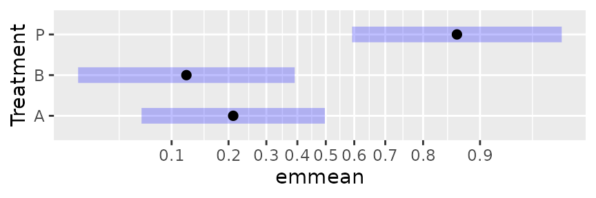

When using the "ggplot" engine, you always have the option of using ggplot2 to incorporate a transformed scale – and it doesn’t even have to be the same as the transformation used in the model. For example, here we display the same results on an arcsin-square-root scale.

plot(neur.Trt.emm, type = "response") +
  ggplot2::scale_x_continuous(trans = scales::asn_trans(),
                              breaks = seq(0.10, 0.90, by = 0.10))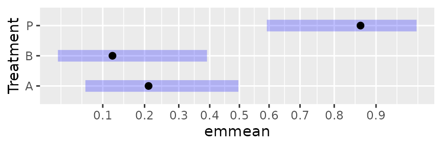

This comes across as a compromise: not as severe as the logit scaling, and not as distorted as the linear scaling of response values.

Again, the same techniques can be used with emmip(), except it is the vertical scale that is affected.

Back to Contents

Models having both a response transformation and a link function

It is possible to have a generalized linear model with a non-identity link and a response transformation. Here is an example, with the built-in wapbreaks dataset:

warp.glm <- glm(sqrt(breaks) ~ wool*tension, family = Gamma, data = warpbreaks)
ref_grid(warp.glm)

## 'emmGrid' object with variables:
##     wool = A, B
##     tension = L, M, H
## Transformation: "inverse" 
## Additional response transformation: "sqrt"

The canonical link for a gamma model is the reciprocal (or inverse); and there is the square-root response transformation besides. If we choose type = "response" in summarizing, we undo both transformations:

emmeans(warp.glm, ~ tension | wool, type = "response")

## wool = A:
##  tension response   SE df lower.CL upper.CL
##  L           42.9 5.24 48     34.0     55.7
##  M           23.3 2.85 48     18.5     30.3
##  H           23.6 2.88 48     18.7     30.7
## 
## wool = B:
##  tension response   SE df lower.CL upper.CL
##  L           27.4 3.35 48     21.8     35.7
##  M           28.1 3.43 48     22.3     36.5
##  H           18.5 2.26 48     14.7     24.1
## 
## Confidence level used: 0.95 
## Intervals are back-transformed from the sqrt[inverse] scale

What happened here is first the linear predictor was back-transformed from the link scale (inverse); then the squares were obtained to back-transform the rest of the way. It is possible to undo the link, and not the response transformation:

emmeans(warp.glm, ~ tension | wool, type = "unlink")

## wool = A:
##  tension response    SE df lower.CL upper.CL
##  L           6.55 0.400 48     5.83     7.46
##  M           4.83 0.295 48     4.30     5.50
##  H           4.86 0.297 48     4.33     5.54
## 
## wool = B:
##  tension response    SE df lower.CL upper.CL
##  L           5.24 0.320 48     4.67     5.97
##  M           5.30 0.324 48     4.72     6.04
##  H           4.30 0.263 48     3.83     4.90
## 
## Confidence level used: 0.95 
## Intervals are back-transformed from the inverse scale

It is not possible to undo the response transformation and leave the link in place, because the response was transform first, then the link model was applied; we have to undo those in reverse order to make sense.

One may also use "unlink" as a transform argument in regrid() or through ref_grid().

Back to Contents

Special transformations

The make.tran() function provides several special transformations and sets things up so they can be handled in emmeans with relative ease. (See help("make.tran", "emmeans") for descriptions of what is available.) make.tran() works much like stats::make.link() in that it returns a list of functions linkfun(), linkinv(), etc. that serve in managing results on a transformed scale. The difference is that most transformations with make.tran() require additional arguments.

To use this capability in emmeans(), it is fortuitous to first obtain the make.tran() result, and then to use it as the enclosing environment for fitting the model, with linkfun as the transformation. For example, suppose the response variable is a percentage and we want to use the response transformation $\sin^{-1}\sqrt{y/100}$. Then proceed like this:

tran <- make.tran("asin.sqrt", 100)
my.model <- with(tran, 
    lmer(linkfun(percent) ~ treatment + (1|Block), data = mydata))

Subsequent calls to ref_grid(), emmeans(), regrid(), etc. will then be able to access the transformation information correctly.

The help page for make.tran() has an example like this using a Box-Cox transformation.

Back to Contents

Specifying a transformation after the fact

It is not at all uncommon to fit a model using statements like the following:

mydata <- transform(mydata, logy.5 = log(yield + 0.5))
my.model <- lmer(logy.5 ~ treatment + (1|Block), data = mydata)

In this case, there is no way for ref_grid() to figure out that a response transformation was used. What can be done is to update the reference grid with the required information:

my.rg <- update(ref_grid(my.model), tran = make.tran("genlog", .5))

Subsequently, use my.rg in place of my.model in any emmeans() analyses, and the transformation information will be there.

For standard transformations (those in stats::make.link()), just give the name of the transformation; e.g.,

model.rg <- update(ref_grid(model), tran = "sqrt")

Auto-detected response transformations

As can be seen in the initial pigs.lm example in this vignette, certain straightforward response transformations such as log, sqrt, etc. are automatically detected when emmeans() (really, ref_grid()) is called on the model object. In fact, scaling and shifting is supported too; so the preceding example with my.model could have been done more easily by specifying the transformation directly in the model formula:

my.better.model <- lmer(log(yield + 0.5) ~ treatment + (1|Block), data = mydata)

The transformation would be auto-detected, saving you the trouble of adding it later. Similarly, a response transformation of 2 * sqrt(y + 1) would be correctly auto-detected. A model with a linearly transformed response, e.g. 4*(y - 1), would not be auto-detected, but 4*I(y + -1) would be interpreted as 4*identity(y + -1). Parsing is such that the response expression must be of the form mult * fcn(resp + const); operators of - and / are not recognized.

Back to Contents

Faking a log transformation

The regrid() function makes it possible to fake a log transformation of the response. Why would you want to do this? So that you can make comparisons using ratios instead of differences.

Consider the pigs example once again, but suppose we had fitted a model with a square-root transformation instead of a log:

pigroot.lm <- lm(sqrt(conc) ~ source + factor(percent), data = pigs)
logemm.src <- regrid(emmeans(pigroot.lm, "source"), transform = "log")
confint(logemm.src, type = "response")

##  source response   SE df lower.CL upper.CL
##  fish       29.8 1.32 23     27.2     32.7
##  soy        39.2 1.54 23     36.2     42.6
##  skim       45.0 1.74 23     41.5     48.7
## 
## Results are averaged over the levels of: percent 
## Confidence level used: 0.95 
## Intervals are back-transformed from the log scale

pairs(logemm.src, type = "response")

##  contrast    ratio     SE df null t.ratio p.value
##  fish / soy  0.760 0.0454 23    1  -4.591  0.0004
##  fish / skim 0.663 0.0391 23    1  -6.965  <.0001
##  soy / skim  0.872 0.0469 23    1  -2.548  0.0457
## 
## Results are averaged over the levels of: percent 
## P value adjustment: tukey method for comparing a family of 3 estimates 
## Tests are performed on the log scale

These results are not identical, but very similar to the back-transformed confidence intervals above for the EMMs and the pairwise ratios in the “comparisons” vignette, where the fitted model actually used a log response.

Faking other transformations

It is possible to fake transformations other than the log. Just use the same method, e.g. (results not displayed)

regrid(emm, transform = "probit")

would re-grid the existing emm to the probit scale. Note that any estimates in emm outside of the interval $(0,1)$ will be flagged as non-estimable.

The section on standardized responses gives an example of reverse-engineering a standardized response transformation in this way.

Revisiting the neuralgia example

As was mentioned before in the neuralgia example, some users prefer ratios of probabilities (risk ratios) rather than odds ratios. The additional machinery of regrid() makes this possible. First, do

log.emm <- regrid(neuralgia.emm, "log")

While each node of neuralgia.emm is an estimate of the logit of a probability, the corresponding nodes of log.emm are estimates of the log of the same probability. Thus, pairwise comparisons are differences of logs, which are logs of ratios. The risk ratios are thus obtainable by

pairs(log.emm, reverse = TRUE, type = "response")

##  contrast ratio    SE  df null z.ratio p.value
##  B / A    0.572 0.484 Inf    1  -0.661  0.7863
##  P / A    4.107 2.220 Inf    1   2.613  0.0244
##  P / B    7.181 5.190 Inf    1   2.730  0.0174
## 
## Results are averaged over the levels of: Sex 
## P value adjustment: tukey method for comparing a family of 3 estimates 
## Tests are performed on the log scale

The test statistics and P values differ somewhat from those for the odds ratios because they are computed on the log scale rather than the original logit scale.

We were able to obtain both odds ratios and risk ratios for neuralgia.glm. But what if we had not used the logit link? Then the odds ratios would not just fall out naturally. However, we can regrid() to the "logit" scale if we want odds ratios, or to "log" scale if we want risk ratios. For example,

neuralgia.prb <- glm(Pain ~ Treatment * Sex + Age, family = binomial(link = "probit"), 
                     data = neuralgia)
prb.emm <- suppressMessages(emmeans(neuralgia.prb, "Treatment"))
pairs(regrid(prb.emm, "logit"), type = "response", reverse = TRUE)

##  contrast odds.ratio     SE  df null z.ratio p.value
##  B / A         0.517  0.509 Inf    1  -0.670  0.7809
##  P / A        15.561 14.400 Inf    1   2.975  0.0082
##  P / B        30.077 33.200 Inf    1   3.081  0.0058
## 
## Results are averaged over the levels of: Sex 
## P value adjustment: tukey method for comparing a family of 3 estimates 
## Tests are performed on the log odds ratio scale

These are vaguely comparable to the odds ratios we obtained with neuralgia.glm, Similar re-gridding for the log will give us risk ratios.

Alternative scale

It is possible to create a report on an alternative scale by updating the tran component. For example, suppose we want percent differences instead of ratios in the preceding example with the pigs dataset. This is possible by modifying the reverse transformation: since the usual reverse transformation is a ratio of the form $r = a/b$, we have that the percentage difference between $a$ and $b$ is $100(a-b)/b = 100(r-1)$. Thus,

pct.diff.tran <- list(
    linkfun = function(mu) log(mu/100 + 1),
    linkinv = function(eta) 100 * (exp(eta) - 1),
    mu.eta = function(eta) 100 * exp(eta),
    name = "log(pct.diff)"
)

update(pairs(logemm.src, type = "response"), 
       tran = pct.diff.tran, inv.lbl = "pct.diff", adjust = "none",
       infer = c(TRUE, TRUE))

##  contrast    pct.diff   SE df lower.CL upper.CL t.ratio p.value
##  fish / soy     -24.0 4.54 23    -32.8   -13.97  -4.591  0.0001
##  fish / skim    -33.7 3.91 23    -41.3   -25.08  -6.965  <.0001
##  soy / skim     -12.8 4.69 23    -22.0    -2.54  -2.548  0.0180
## 
## Results are averaged over the levels of: percent 
## Confidence level used: 0.95 
## Intervals are back-transformed from the log(pct.diff) scale 
## Tests are performed on the log(pct.diff) scale

Another way to obtain the same estimates is to directly transform the estimated ratios to $100r - 100$:

contrast(regrid(pairs(logemm.src)), "identity", scale = 100, offset = -100,
         infer = c(TRUE, TRUE))

##  contrast    estimate   SE df lower.CL upper.CL t.ratio p.value
##  (fish/soy)     -24.0 4.54 23    -33.3    -14.6  -5.281  <.0001
##  (fish/skim)    -33.7 3.91 23    -41.8    -25.6  -8.613  <.0001
##  (soy/skim)     -12.8 4.69 23    -22.5     -3.1  -2.730  0.0119
## 
## Results are averaged over the levels of: percent 
## Confidence level used: 0.95

While the estimates are the same, the tests and confidence intervals are different because they are computed on the re-gridded scale using the standard errors shown, rather than on the link scale as in the first results.

Standardized response

In some disciplines, it is common to fit a model to a standardized response variable. R’s base function scale() makes this easy to do; but it is important to notice that scale(y) is more complicated than, say, sqrt(y), because scale(y) requires all the values of y in order to determine the centering and scaling parameters. The ref_grid() function (called by `emmeans() and others) tries to detect the scaling parameters. To illustrate:

fiber.lm <- lm(scale(strength) ~ machine * scale(diameter), data = fiber)
emmeans(fiber.lm, "machine")   # on the standardized scale

##  machine   emmean    SE df lower.CL upper.CL
##  A        0.00444 0.156  9   -0.349    0.358
##  B        0.28145 0.172  9   -0.109    0.672
##  C       -0.33473 0.194  9   -0.774    0.105
## 
## Results are given on the scale(40.2, 4.97) (not the response) scale. 
## Confidence level used: 0.95

emmeans(fiber.lm, "machine", type = "response")   # strength scale

##  machine response    SE df lower.CL upper.CL
##  A           40.2 0.777  9     38.5     42.0
##  B           41.6 0.858  9     39.7     43.5
##  C           38.5 0.966  9     36.3     40.7
## 
## Confidence level used: 0.95 
## Intervals are back-transformed from the scale(40.2, 4.97) scale

More interesting (and complex) is what happens with emtrends(). Without anything fancy added, we have

emtrends(fiber.lm, "machine", var = "diameter")

##  machine diameter.trend     SE df lower.CL upper.CL
##  A                0.222 0.0389  9   0.1339    0.310
##  B                0.172 0.0450  9   0.0705    0.274
##  C                0.174 0.0418  9   0.0791    0.268
## 
## Confidence level used: 0.95

These slopes are (change in scale(strength)) / (change in diameter); that is, we didn’t do anything to undo the response transformation, but the trend is based on exactly the variable specified, diameter. To get (change in strength) / (change in diameter), we need to undo the response transformation, and that is done via regrid (which invokes regrid() after the reference grid is constructed):

emtrends(fiber.lm, "machine", var = "diameter", regrid = "response")

##  machine diameter.trend    SE df lower.CL upper.CL
##  A                1.104 0.194  9    0.666     1.54
##  B                0.857 0.224  9    0.351     1.36
##  C                0.864 0.208  9    0.394     1.33
## 
## Confidence level used: 0.95

What if we want slopes for (change in scale(strength)) / (change in scale(diameter))? This can be done, but it is necessary to manually specify the scaling parameters for diameter.

with(fiber, c(mean = mean(diameter), sd = sd(diameter)))

##      mean        sd 
## 24.133333  4.323799

emtrends(fiber.lm, "machine", var = "scale(diameter, 24.133, 4.324)")

##  machine scale(diameter, 24.133, 4.324).trend    SE df lower.CL upper.CL
##  A                                      0.960 0.168  9    0.579     1.34
##  B                                      0.745 0.195  9    0.305     1.19
##  C                                      0.751 0.181  9    0.342     1.16
## 
## Confidence level used: 0.95

This result is the one most directly related to the regression coefficients:

coef(fiber.lm)[4:6]

##          scale(diameter) machineB:scale(diameter) machineC:scale(diameter) 
##                0.9598846               -0.2148202               -0.2086880

There is a fourth possibility, (change in strength) / (change in scale(diameter)), that I leave to the reader.

What to do if auto-detection fails

Auto-detection of standardized responses is a bit tricky, and doesn’t always succeed. If it fails, a message is displayed and the transformation is ignored. In cases where it doesn’t work, we need to explicitly specify the transformation using make.tran(). The methods are exactly as shown earlier in this vignette, so we show the code but not the results for a hypothetical example.

One method is to fit the model and then add the transformation information later. In this example, some.fcn is a model-fitting function which for some reason doesn’t allow the scaling information to be detected.

mod <- some.fcn(scale(RT) ~ group + (1|subject), data = mydata)
emmeans(mod, "group", type = "response",
        tran = make.tran("scale", y = mydata$RT))

The other, equivalent, method is to create the transformation object first and use it in fitting the model:

mod <- with(make.tran("scale", y = mydata$RT),
            some.fcn(linkfun(RT) ~ group + (1|subject), data = mydata))
emmeans(mod, "group", type = "response")

Reverse-engineering a standardized response

An interesting twist on all this is the reverse situation: Suppose we fitted the model without the standardized response, but we want to know what the results would be if we had standardized. Here we reverse-engineer the fiber.lm example above:

fib.lm <- lm(strength ~ machine * diameter, data = fiber)

# On raw scale:
emmeans(fib.lm, "machine")

##  machine emmean    SE df lower.CL upper.CL
##  A         40.2 0.777  9     38.5     42.0
##  B         41.6 0.858  9     39.7     43.5
##  C         38.5 0.966  9     36.3     40.7
## 
## Confidence level used: 0.95

# On standardized scale:
tran <- make.tran("scale", y = fiber$strength)
emmeans(fib.lm, "machine", regrid = tran)

##  machine   emmean    SE df lower.CL upper.CL
##  A        0.00444 0.156  9   -0.349    0.358
##  B        0.28145 0.172  9   -0.109    0.672
##  C       -0.33473 0.194  9   -0.774    0.105
## 
## Results are given on the scale(40.2, 4.97) (not the response) scale. 
## Confidence level used: 0.95

In the latter call, the regrid argument causes regrid() to be called after the reference grid is constructed.

Back to Contents

Bias adjustment

So far, we have discussed ideas related to back-transforming results as a simple way of expressing results on the same scale as the response. In particular, means obtained in this way are known as generalized means; for example, a log transformation of the response is associated with geometric means. When the goal is simply to make inferences about which means are less than which other means, and a response transformation is used, it is often acceptable to present estimates and comparisons of these generalized means. However, sometimes it is important to report results that actually do reflect expected values of the untransformed response. An example is a financial study, where the response is in some monetary unit. It may be convenient to use a response transformation for modeling purposes, but ultimately we may want to make financial projections in those same units.

In such settings, we need to make a bias adjustment when we back-transform, because any nonlinear transformation biases the expected values of statistical quantities. More specifically, suppose that we have a response $Y$ and the transformed response is $U$. To back-transform, we use $Y = h(U)$; and using a Taylor approximation, $Y \approx h(\eta) + h'(\eta)(U-\eta) + \frac12h''(\eta)(U-\eta)^2$, so that $E(Y) \approx h(\eta) + \frac12h''(\eta)Var(U)$. This shows that the amount of needed bias adjustment is approximately $\frac12h''(\eta)\sigma^2$ where $\sigma$ is the error SD in the model for $U$. It depends on $\sigma$, and the larger this is, the greater the bias adjustment is needed. This second-order bias adjustment is what is currently used in the emmeans package when bias-adjustment is requested. There are better or exact adjustments for certain cases, and future updates may incorporate some of those.

Pigs example revisited

Let us compare the estimates in the overview after we apply a bias adjustment. First, note that an estimate of the residual SD is available via the sigma() function:

sigma(pigs.lm)

## [1] 0.115128

This estimate is used by default. The bias-adjusted EMMs for the sources are:

summary(emm.src, type = "response", bias.adj = TRUE)

##  source response   SE df lower.CL upper.CL
##  fish       30.0 1.10 23     27.8     32.4
##  soy        39.4 1.48 23     36.5     42.6
##  skim       44.9 1.77 23     41.3     48.7
## 
## Results are averaged over the levels of: percent 
## Confidence level used: 0.95 
## Intervals are back-transformed from the log scale 
## Bias adjustment applied based on sigma = 0.11513

These estimates (and also their SEs) are slightly larger than we had without bias adjustment. They are estimates of the arithmetic mean responses, rather than the geometric means shown in the overview. Had the value of sigma been larger, the adjustment would have been greater. You can experiment with this by adding a sigma = argument to the above call.

Response transformations vs. link functions

At this point, it is important to point out that the above discussion focuses on response transformations, as opposed to link functions used in generalized linear models (GLMs). In an ordinary GLM, no bias adjustment is needed, nor is it appropriate, because the link function is just used to define a nonlinear relationship between the actual response mean $\eta$ and the linear predictor. That is, the back-transformed parameter is already the mean.

InsectSprays example

To illustrate this, consider the InsectSprays data in the datasets package. The response variable is a count, and there is one treatment, the spray that is used. Let us model the count as a Poisson variable with (by default) a log link; and obtain the EMMs, with and without a bias adjustment

ismod <- glm(count ~ spray, data = InsectSprays, family = poisson())
emmeans(ismod, "spray", type = "response")

##  spray  rate    SE  df asymp.LCL asymp.UCL
##  A     14.50 1.100 Inf     12.50     16.82
##  B     15.33 1.130 Inf     13.27     17.72
##  C      2.08 0.417 Inf      1.41      3.08
##  D      4.92 0.640 Inf      3.81      6.35
##  E      3.50 0.540 Inf      2.59      4.74
##  F     16.67 1.180 Inf     14.51     19.14
## 
## Confidence level used: 0.95 
## Intervals are back-transformed from the log scale

The above results were computed with no bias adjustment, the default. If you try

emmeans(ismod, "spray", type = "response", bias.adj = TRUE)

you will get exactly the same results, plus a warning message that says bias adjustment was disabled. Why? Because in an ordinary GLM like this, we are already modeling the mean counts, and the link function is not a response transformation as such, just a part of the relationship we are specifying between the linear predictor and the mean. Given the simple structure of this dataset, we can verify this by noting that the estimates we have correspond exactly to the simple observed mean counts:

with(InsectSprays, tapply(count, spray, mean))

##         A         B         C         D         E         F 
## 14.500000 15.333333  2.083333  4.916667  3.500000 16.666667

The point here is that a GLM does not have an additive error term, that the model is already formulated in terms of the mean, not some generalized mean. (You can enable the bias-adjustment computations by specifying a valid sigma value; but you should not do so.)

Note that, in a generalized linear mixed model, including generalized estimating equations and such, there are additive random components involved, and then bias adjustment becomes appropriate.

CBPP example

Consider an example adapted from the help page for lme4::cbpp. Contagious bovine pleuropneumonia (CBPP) is a disease in African cattle, and the dataset contains data on incidence of CBPP in several herds of cattle over four time periods. We will fit a mixed model that accounts for herd variations as well as overdispersion (variations larger than expected with a simple binomial model):

require(lme4)
cbpp <- transform(cbpp, unit = 1:nrow(cbpp))
cbpp.glmer <- glmer(cbind(incidence, size - incidence) ~ period + 
                          (1 | herd) +  (1 | unit),
                    family = binomial, data = cbpp)

emm <- emmeans(cbpp.glmer, "period")
summary(emm, type = "response")

##  period   prob     SE  df asymp.LCL asymp.UCL
##  1      0.1824 0.0442 Inf    0.1109    0.2852
##  2      0.0614 0.0230 Inf    0.0290    0.1252
##  3      0.0558 0.0220 Inf    0.0254    0.1182
##  4      0.0334 0.0172 Inf    0.0120    0.0894
## 
## Confidence level used: 0.95 
## Intervals are back-transformed from the logit scale

The above summary reflects the back-transformed estimates, with no bias adjustment. However, the model estimates two independent sources of random variation that probably should be taken into account:

lme4::VarCorr(cbpp.glmer)

##  Groups Name        Std.Dev.
##  unit   (Intercept) 0.89107 
##  herd   (Intercept) 0.18396

Notably, the over-dispersion SD is considerably greater than the herd SD. Suppose we want to estimate the marginal probabilities of CBPP incidence, averaged over herds and over-dispersion variations. For this purpose, we need the combined effect of these variations; so we compute the overall SD via the Pythagorean theorem:

total.SD = sqrt(0.89107^2 + 0.18396^2)

Accordingly, here are the bias-adjusted estimates of the marginal probabilities:

summary(emm, type = "response", bias.adjust = TRUE, sigma = total.SD)

##  period   prob     SE  df asymp.LCL asymp.UCL
##  1      0.2216 0.0462 Inf    0.1426     0.321
##  2      0.0823 0.0292 Inf    0.0400     0.159
##  3      0.0751 0.0282 Inf    0.0351     0.151
##  4      0.0458 0.0230 Inf    0.0168     0.117
## 
## Confidence level used: 0.95 
## Intervals are back-transformed from the logit scale 
## Bias adjustment applied based on sigma = 0.90986

These estimates are somewhat larger than the unadjusted estimates (actually, any estimates greater than 0.5 would have been adjusted downward). These adjusted estimates are more appropriate for describing the marginal incidence of CBPP for all herds. In fact, these estimates are fairly close to those obtained directly from the incidences in the data:

cases <- with(cbpp, tapply(incidence, period, sum))
trials <- with(cbpp, tapply(size, period, sum))
cases / trials

##          1          2          3          4 
## 0.21942446 0.08018868 0.07106599 0.04516129

Left as an exercise: Revisit the InsectSprays example, but (using similar methods to the above) create a unit variable and fit an over-dispersion model. Compare the results with and without bias adjustment, and evaluate these results against the earlier results. This is simpler than the CBPP example because there is only one random effect.

Back to Contents

Index of all vignette topics