Construct an emmGrid object from scratch

This allows the user to incorporate results obtained by some analysis into an emmGrid object, enabling the use of emmGrid methods to perform related follow-up analyses.

Usage

emmobj(bhat, V, levels, linfct = diag(length(bhat)), df = NA, dffun,
  dfargs = list(), post.beta = matrix(NA), nesting = NULL, se.bhat,
  se.diff, ...)

Arguments

bhat

Numeric. Vector of regression coefficients

V

Square matrix. Covariance matrix of bhat

levels

Named list or vector. Levels of factor(s) that define the estimates defined by linfct. If not a list, we assume one factor named "level"

linfct

Matrix. Linear functions of bhat for each combination of levels.

df

Numeric value or function with arguments (x, dfargs). If a number, that is used for the degrees of freedom. If a function, it should return the degrees of freedom for sum(x*bhat), with any additional parameters in dfargs.

dffun

Overrides df if specified. This is a convenience to match the slot names of the returned object.

dfargs

List containing arguments for df. This is ignored if df is numeric.

post.beta

Matrix whose columns comprise a sample from the posterior distribution of the regression coefficients (so that typically, the column averages will be bhat). A 1 x 1 matrix of NA indicates that such a sample is unavailable.

nesting

Nesting specification as in ref_grid. This is ignored if model.info is supplied.

se.bhat, se.diff

Alternative way of specifying V. If se.bhat is specified, V is constructed using se.bhat, the standard errors of bhat, and se.diffs, the standard errors of its pairwise differences. se.diff should be a vector of length k*(k-1)/2 where k is the length of se.bhat, and its elements should be in the order 12,13,...,1k,23,...2k,.... If se.diff is missing, V is computed as if the bhat are independent.

...

Arguments passed to update.emmGrid

Value

An emmGrid object

Details

The arguments must be conformable. This includes that the length of bhat, the number of columns of linfct, and the number of columns of post.beta must all be equal. And that the product of lengths in levels must be equal to the number of rows of linfct. The grid slot of the returned object is generated by expand.grid using levels as its arguments. So the rows of linfct should be in corresponding order.

The functions qdrg and emmobj are close cousins, in that they both produce emmGrid objects. When starting with summary statistics for an existing grid, emmobj is more useful, while qdrg is more useful when starting from an unsupported fitted model.

See also

qdrg, an alternative that is useful when starting with a fitted model not supported in emmeans.

Examples

# Given summary statistics for 4 cells in a 2 x 2 layout, obtain 
# marginal means and comparisons thereof. Assume heteroscedasticity
# and use the Satterthwaite method
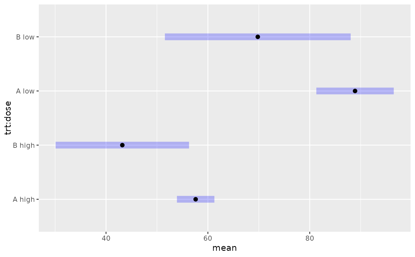
levels <- list(trt = c("A", "B"), dose = c("high", "low"))
ybar <- c(57.6, 43.2, 88.9, 69.8)
s <-    c(12.1, 19.5, 22.8, 43.2)
n <-    c(44,   11,   37,   24)
se2 = s^2 / n
Satt.df <- function(x, dfargs)
    sum(x * dfargs$v)^2 / sum((x * dfargs$v)^2 / (dfargs$n - 1))
    
expt.emm <- emmobj(bhat = ybar, V = diag(se2),
    levels = levels, linfct = diag(c(1, 1, 1, 1)),
    df = Satt.df, dfargs = list(v = se2, n = n), estName = "mean")

( trt.emm <- emmeans(expt.emm, "trt") )
#>  trt mean   SE   df lower.CL upper.CL
#>  A   73.2 2.08 52.6     69.1     77.4
#>  B   56.5 5.30 33.0     45.7     67.3
#> 
#> Results are averaged over the levels of: dose 
#> Confidence level used: 0.95 
( dose.emm <- emmeans(expt.emm, "dose") )
#>  dose mean   SE   df lower.CL upper.CL
#>  high 50.4 3.08 12.0     43.7     57.1
#>  low  79.3 4.79 31.4     69.6     89.1
#> 
#> Results are averaged over the levels of: trt 
#> Confidence level used: 0.95 

rbind(pairs(trt.emm), pairs(dose.emm), adjust = "mvt")
#>  contrast   estimate   SE    df t.ratio p.value
#>  A - B          16.8 5.69 23.23   2.941  0.0143
#>  high - low    -28.9 5.69  7.49  -5.084  0.0027
#> 
#> Results are averaged over some or all of the levels of: dose, trt 
#> P value adjustment: mvt method for 2 tests 

### Create an emmobj from means and SEs
### (This illustration reproduces the MOats example for Variety = "Victory")
means = c(71.50000,  89.66667, 110.83333, 118.50000)
semeans = c(5.540591, 6.602048, 8.695358, 7.303221)
sediffs = c(7.310571,  9.894724,  7.463615, 10.248306,  4.935698,  8.694507)
foo = emmobj(bhat = means, se.bhat = semeans, se.diff = sediffs, 
             levels = list(nitro = seq(0, .6, by = .2)), df = 10)
plot(foo, comparisons = TRUE)