Feedlot data

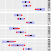
This is an unbalanced analysis-of-covariance example, where one covariate is affected by a factor. Feeder calves from various herds enter a feedlot, where they are fed one of three diets. The weight of the animal at entry is the covariate, and the weight at slaughter is the response.

Usage

feedlot

Format

A data frame with 67 observations and 4 variables:

herd

a factor with levels 9 16 3 32 24 31 19 36 34 35 33, designating the herd that a feeder calf came from.

diet

a factor with levels Low Medium High: the energy level of the diet given the animal.

swt

a numeric vector: the weight of the animal at slaughter.

ewt

a numeric vector: the weight of the animal at entry to the feedlot.

Source

Urquhart NS (1982) Adjustment in covariates when one factor affects the covariate. Biometrics 38, 651-660.

Details

The data arise from a Western Regional Research Project conducted at New Mexico State University. Calves born in 1975 in commercial herds entered a feedlot as yearlings. Both diets and herds are of interest as factors. The covariate, ewt, is thought to be dependent on herd due to different genetic backgrounds, breeding history, etc. The levels of herd ordered to similarity of genetic background.

Note: There are some empty cells in the cross-classification of herd and diet.

Examples

feedlot.lm <- lm(swt ~ ewt + herd*diet, data = feedlot)

# Obtain EMMs with a separate reference value of ewt for each 
# herd. This reproduces the last part of Table 2 in the reference
emmeans(feedlot.lm,  ~ diet | herd,  cov.reduce = ewt ~ herd)
#> herd = 9:
#>  diet   emmean   SE df lower.CL upper.CL
#>  Low       839 32.7 36      773      906
#>  Medium    877 40.1 36      796      958
#>  High   nonEst   NA NA       NA       NA
#> 
#> herd = 16:
#>  diet   emmean   SE df lower.CL upper.CL
#>  Low       940 41.3 36      856     1024
#>  Medium    951 60.3 36      829     1073
#>  High   nonEst   NA NA       NA       NA
#> 
#> herd = 3:
#>  diet   emmean   SE df lower.CL upper.CL
#>  Low       981 32.8 36      915     1048
#>  Medium   1002 41.2 36      918     1085
#>  High     1015 63.5 36      886     1144
#> 
#> herd = 32:
#>  diet   emmean   SE df lower.CL upper.CL
#>  Low      1003 33.2 36      936     1070
#>  Medium    890 40.2 36      809      972
#>  High      970 32.9 36      904     1037
#> 
#> herd = 24:
#>  diet   emmean   SE df lower.CL upper.CL
#>  Low       982 28.3 36      924     1039
#>  Medium    982 32.7 36      916     1048
#>  High   nonEst   NA NA       NA       NA
#> 
#> herd = 31:
#>  diet   emmean   SE df lower.CL upper.CL
#>  Low      1128 32.9 36     1062     1195
#>  Medium   1069 40.4 36      987     1151
#>  High     1111 56.6 36      996     1226
#> 
#> herd = 19:
#>  diet   emmean   SE df lower.CL upper.CL
#>  Low      1087 28.3 36     1030     1145
#>  Medium   1036 40.0 36      955     1117
#>  High      999 56.7 36      884     1114
#> 
#> herd = 36:
#>  diet   emmean   SE df lower.CL upper.CL
#>  Low      1155 40.5 36     1073     1237
#>  Medium   1062 41.3 36      978     1146
#>  High     1191 57.2 36     1075     1307
#> 
#> herd = 34:
#>  diet   emmean   SE df lower.CL upper.CL
#>  Low       987 33.6 36      918     1055
#>  Medium   1015 41.0 36      931     1098
#>  High     1048 40.1 36      967     1129
#> 
#> herd = 35:
#>  diet   emmean   SE df lower.CL upper.CL
#>  Low      1094 29.1 36     1035     1153
#>  Medium   1092 41.8 36     1008     1177
#>  High     1103 40.0 36     1021     1184
#> 
#> herd = 33:
#>  diet   emmean   SE df lower.CL upper.CL
#>  Low      1207 57.3 36     1091     1323
#>  Medium   1031 32.7 36      964     1097
#>  High     1018 56.6 36      903     1133
#> 
#> Confidence level used: 0.95