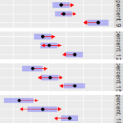
Fiber data from Montgomery Design (8th ed.), p.656 (Table 15.10). Useful as a simple analysis-of-covariance example.
Format
A data frame with 15 observations and 3 variables:
machinea factor with levels
ABC. This is the primary factor of interest.strengtha numeric vector. The response variable.
diametera numeric vector. A covariate.
Source
Montgomery, D. C. (2013) Design and Analysis of Experiments (8th ed.). John Wiley and Sons, ISBN 978-1-118-14692-7.
Details
The goal of the experiment is to compare the mean breaking strength of fibers produced by the three machines. When testing this, the technician also measured the diameter of each fiber, and this measurement may be used as a concomitant variable to improve precision of the estimates.
Examples
fiber.lm <- lm(strength ~ diameter + machine, data=fiber)
ref_grid(fiber.lm)
#>  diameter machine prediction    SE df
#>      24.1 A             40.4 0.724 11
#>      24.1 B             41.4 0.744 11
#>      24.1 C             38.8 0.788 11
#>

# Covariate-adjusted means and comparisons
emmeans(fiber.lm, pairwise ~ machine)
#> $emmeans
#>  machine emmean    SE df lower.CL upper.CL
#>  A         40.4 0.724 11     38.8     42.0
#>  B         41.4 0.744 11     39.8     43.1
#>  C         38.8 0.788 11     37.1     40.5
#>
#> Confidence level used: 0.95
#>
#> $contrasts
#>  contrast estimate   SE df t.ratio p.value
#>  A - B       -1.04 1.01 11  -1.024  0.5781
#>  A - C        1.58 1.11 11   1.431  0.3596
#>  B - C        2.62 1.15 11   2.283  0.1005
#>
#> P value adjustment: tukey method for comparing a family of 3 estimates
#>
