Sales of oranges — oranges • emmeans

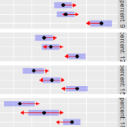
This example dataset on sales of oranges has two factors, two covariates, and two responses. There is one observation per factor combination.

Usage

oranges

Format

A data frame with 36 observations and 6 variables:

store: a factor with levels 1 2 3 4 5 6. The store that was observed.
day: a factor with levels 1 2 3 4 5 6. The day the observation was taken (same for each store).
price1: a numeric vector. Price of variety 1.
price2: a numeric vector. Price of variety 2.
sales1: a numeric vector. Sales (per customer) of variety 1.
sales2: a numeric vector. Sales (per customer) of variety 2.

Source

This is (or once was) available as a SAS sample dataset.

References

Littell, R., Stroup W., Freund, R. (2002) SAS For Linear Models (4th edition). SAS Institute. ISBN 1-59047-023-0.

Examples

# Example on p.244 of Littell et al.
oranges.lm <- lm(sales1 ~ price1*day, data = oranges)
emmeans(oranges.lm, "day")
#> NOTE: Results may be misleading due to involvement in interactions
#>  day emmean   SE df lower.CL upper.CL
#>  1     7.38 2.01 24     3.23     11.5
#>  2     6.55 1.92 24     2.58     10.5
#>  3    14.03 1.92 24    10.07     18.0
#>  4     8.40 1.91 24     4.46     12.3
#>  5    16.65 2.47 24    11.55     21.7
#>  6    10.51 1.92 24     6.55     14.5
#> 
#> Confidence level used: 0.95 

# Example on p.246 of Littell et al.
emmeans(oranges.lm, "day", at = list(price1 = 0))
#> NOTE: Results may be misleading due to involvement in interactions
#>  day emmean   SE df lower.CL upper.CL
#>  1     18.7 14.4 24   -11.07     48.4
#>  2     38.5 15.1 24     7.30     69.7
#>  3     45.3 26.2 24    -8.66     99.3
#>  4     49.1 16.6 24    14.87     83.4
#>  5     77.9 27.5 24    21.14    134.7
#>  6     73.3 13.5 24    45.44    101.1
#> 
#> Confidence level used: 0.95 

# A more sensible model to consider, IMHO (see vignette("interactions"))
org.mlm <- lm(cbind(sales1, sales2) ~ price1 * price2 + day + store, 
              data = oranges)